Notes on Abstract Interpretation
This is my notes on abstract interpretation based on Bruno Blanchet’s Introduction to Abstract Interpretation, Matt Might’s blog post Order theory for computer scientists, Alexandru Salcianu’s Notes on Abstract Interpretation, and Stephen Chong’s CS252r course material.
1 Motivation
Most of the interesting properties of programs are undecidable since they can be reduced to the Halting Problem. The proof of undecidability of Halting problem is as follows.
Proof: By contradiction. First assume that there existing an analyzer Halt?(P, E) returning true when program P terminates on input E and false otherwise. Consider a program Q(P) = if Halt?(P, P) then loop else halt. Now apply Q(Q):
If Halt?(Q, Q) is true, then Q(Q) loops. Contradiction.
If Halt?(Q, Q) is false, then Q(Q) halts. Contradiction. □
To analyze the behavior of programs, we introduce approximations. The approximations must be sound: if the system gives a definite answer, then this answer is true. Sometimes the system answers “maybe”, then the system is not complete.
2 A Simple Language
In this simple programming language, a program is a function from integers (PC) to commands, indicating the command at each PC in the program.
2.1 Syntax
We define the grammar of expressions:
| ‹Exp› | ::= | ‹var› |
|
| | | ‹num› |
|
| | | ‹Exp› ‹Aop› ‹Exp› |
|
| | | ‹Exp› ‹Bop› ‹Exp› |
| ‹Aop› | ::= | + |
|
| | | - |
|
| | | * |
|
| | | / |
| ‹Bop› | ::= | >= |
|
| | | ... |
and the grammar of commands:
| ‹Cmd› | ::= | ‹var› := ‹Exp› |
|
| | | if ‹Exp› goto ‹PC› |
|
| | | input ‹var› |
|
| | | print ‹Exp› |
|
| | | abort |
2.2 Trace Semantics
The state of programs consists of 1) a program counter, which indicates the next command to execute, 2) an environment, which contains a partial map from variables to values. We ignore overflows. Formally,
pc \in PC := \mathbb{N} \rho \in Env := Var \rightarrow \mathbb{Z} s \in State := PC \times Env
The semantics of expressions is a function \llbracket Exp \rrbracket \rho \in \mathbb{Z}. In case of errors (e.g., division by 0), \llbracket Exp \rrbracket \rho is undefined. We may use \bot to represent that.
- The semantics of commands is modeled as a transition system: \langle pc, \rho \rangle \rightarrow \langle pc{}’, \rho{}’ \rangle. Now given a program P, and current state \langle pc, \rho \rangle,
If P(pc) = x := E, then \langle pc, \rho \rangle \rightarrow \langle pc+1, \rho[ x \mapsto \llbracket E \rrbracket \rho ] \rangle, if \llbracket E \rrbracket \rho is defined
If P(pc) = if E goto n, then \langle pc, \rho \rangle \rightarrow \langle n, \rho \rangle if \llbracket E \rrbracket \rho \neq 0; \langle pc, \rho \rangle \rightarrow \langle pc+1, \rho \rangle otherwise.
If P(pc) = input x, then \langle pc, \rho \rangle \rightarrow \langle pc+1, \rho[ x \mapsto v ] \rangle for some v \in \mathbb{Z}.
If P(pc) = print E, then \langle pc, \rho \rangle \rightarrow \langle pc+1, \rho \rangle if \llbracket E \rrbracket \rho is defined.
A sequence of states is a trace. A program may have several traces, depending on the user input; so the semantics of a program is a set of traces.
3 Theory of Approximation
We want to prove properties like “all traces of the program satisfy a given condition”. To do this, we over-approximate the set of traces, and obtain a superset of the set of concrete traces. An analysis is more precise when it yields a small superset of the set of concrete traces. All correct approximations are the ones are greater than the smallest correct one, namely, the set of concrete traces.
3.1 Order, Lattices, and Complete Lattices
Definition (Partially-ordered set): A partially-ordered set (poset for short) is a set S equipped with a binary relation \leq which is reflexive, anti-symmetric and transitive. A binary relation R is anti-symmetric if a R b and b R a implies a = b.
c \in S is an upper bound of X \subseteq S iff \forall c{}’ \in X, c{}’ \leq c.
c \in S is a lower bound of X \subseteq S iff \forall c{}’ \in X, c \leq c{}’.
c \in S is the least upper bound of X \subseteq S iff \forall c{}’ \in X, c{}’ \leq c and \forall c{}’{}’ \in S s.t. \forall c{}’ \in X, c{}’ \leq c{}’{}’, we have c \leq c{}’{}’.
c \in S is the greatest lower bound of X \subseteq S iff \forall c{}’ \in X, c \leq c{}’ and \forall c{}’{}’ \in S s.t. \forall c{}’ \in X, c{}’{}’ \leq c{}’, we have c{}’{}’ \leq c.
The ordering relation can be partial, i.e., there exists incomparable elements.
Definition (Lattice): A lattice is a poset (L, \leq) s.t. for all a, b \in L, a and b have a least upper bound a \sqcup b and a greatest lower bound a \sqcap b. We denote the lattice by (L, \leq, \sqcup, \sqcap).
All finite sets in a lattice have least upper bounds and greatest lower bounds, but not necessarily for infinite sets.
Definition (Complete lattice): A complete lattice is a poset (L, \leq) s.t. every subset X of L has a least upper bound \sqcup X and a greatest lower bound \sqcap X. In particular, L has a least element \bot = \sqcup \varnothing and a greatest element \top = \sqcap L. We denote the complete lattice by (L, \leq, \bot, \top, \sqcup, \sqcap).
Proposition: If S is a set, then (\mathcal{P}(S), \subseteq, \varnothing, S, \cup, \cap) is a complete lattice.
Intuitively, a \leq b means that a is more precise than b.
3.2 Collecting Semantics
Collecting semantics computes the set of possible traces, formally:
T_r = \{ s_1 \rightarrow \cdots \rightarrow s_n | s_1 \text{ is the initial state,}~ s_i \rightarrow s_{i+1} ~\text{is an allowed transition} \}
The set of reachable states is defined by:
S_r = \{ s | s_1 \rightarrow \cdots \rightarrow s \in T_r \}
The set of all traces, of all states, are ordered by inclusion. They are complete lattice (in this case, they are concrete lattice.)
4 Galois Connections
Definition (Galois connection): Let (L_1, \leq_1) and (L_2, \leq_2) be posets. (\alpha, \gamma) is a Galois connection (or pair of adjoined functions) between L_1 and L_2 iff \alpha : L_1 \to L_2 and \gamma : L_2 \to L_1, and \forall x \in L_1, \forall y \in L_2, \alpha(x) \leq_2 y \iff x \leq_1 \gamma(y)
4.1 Examples
The concrete lattice is (\mathcal{P}(S), \subseteq) for some set S. The abstract lattice contains elements \bot, c, \top; for each c \in S, ordered by \bot \leq c \leq \top. The abstraction is defined by \alpha(\varnothing) = \bot, \alpha(\{c\}) = c, \alpha(\_) = \top. The concretization is defined by \gamma(\bot) = \varnothing, \gamma(c) = \{c\}, \gamma(\top) = S.
Sign. The concrete lattice is \mathcal{P}(\mathbb{Z}). The abstract lattice is \mathcal{P}(\{-, 0, +\}), ordered by inclusion. The abstraction is defined by: \alpha(S) = \begin{cases} \{+\}, & \text{if }S \cap [0, +\infty] \neq \varnothing \\ \{0\}, & \text{if }0 \in S \\ \{-\}, & \text{if }S \cap [-\infty, 0] \neq \varnothing \end{cases} The concretization is defined by: \gamma(\hat{S}) = \begin{cases} [-\infty, 0], & \text{if } - \in \hat{S} \\ \{0\} , & \text{if } 0 \in \hat{S} \\ [0, +\infty], & \text{if } + \in \hat{S} \end{cases}
Interval. The concrete lattice is \mathcal{P}(\mathbb{Z}). The abstract lattice is \{ \varnothing \} \cup \{ [a, b] | a \leq b, a \in \mathbb{Z} \cup \{- \infty\}, b \in \mathbb{Z} \cup \{+\infty\} \} The ordering is [a,b] \leq [a{}’,b{}’] iff a{}’ \leq a and b \leq b{}’; additionally, \varnothing \leq [a, b]. The abstraction is defined by: \alpha(S) = \begin{cases} \varnothing, & \text{if } S = \varnothing \\ [min(S), max(S)], & \text{otherwise} \end{cases} The concretization is defined by: \gamma(\hat{S}) = \begin{cases} \varnothing, & \text{if } \hat{S} = \varnothing \\ \{a, \dots, b\}, & \text{if } \hat{S} = [a,b] \end{cases}
4.2 Properties
Proposition: (\alpha, \gamma) is a Glaois connection iff \alpha and \gamma are monotone, (\alpha \circ \gamma)(y) \leq_2 y and x \leq_1 (\gamma \circ \alpha)(x).
Proof:
By definition \alpha(x) \leq_2 y, and by reflexivity \gamma(y) \leq_1 \gamma(y), thus (\alpha \circ \gamma)(y) \leq_2 y.
By definition x \leq_1 \gamma(y), and by reflexivity \alpha(x) \leq_2 \alpha(x), thus x \leq_1 (\gamma \circ \alpha)(y).
Let x \leq_1 x{}’. We know that x{}’ \leq_1 (\gamma \circ \alpha)(x{}’), then by transitivity, x \leq_1 (\gamma \circ \alpha)(x{}’). Thus by definition, \alpha(x) \leq_2 \alpha(x{}’), and \alpha is monotone.
Let y \leq_2 y{}’. We know that (\alpha \circ \gamma)(y) \leq_2 y, then by transitivity, (\alpha \circ \gamma)(y) \leq_2 y{}’. Thus by definition, \gamma(y) \leq_2 \gamma(y{}’), and \gamma is monotone.
Assume that \alpha(x) \leq_2 y, since \gamma is monotone, then \gamma(\alpha(x)) \leq_1 \gamma(y). By assumption, x \leq_1 \gamma(\alpha(x)); by transitivity, x \leq_1 \gamma(y).
Assume that x \leq_1 \gamma(y), since \alpha is monotone, then \alpha(x) \leq_2 \alpha(\gamma(y)). By assumption, \alpha(\gamma(y)) \leq_2 y; by transitivity, \alpha(x) \leq_2 y. □
Proposition: Let (L_1, \leq_1, \bot_1, \top_1, \sqcup_1, \sqcap_1) and (L_2, \leq_2, \bot_2, \top_2, \sqcup_2, \sqcap_2) be complete lattices, and (\alpha, \gamma) be a Galois connection between L_1 and L_2. Then
Each function in the pair (\alpha, \gamma) uniquely determines the other: \alpha(x) = \sqcap_2 \{ y \in L_2 \mid x \leq_1 \gamma(y) \} \\ \gamma(y) = \sqcup_1 \{ x \in L_1 | \alpha(x) \leq_2 y\}
\alpha is a complete join-morphism (i.e., additive: \alpha(\sqcup_1 S) = \sqcup_2 \{ \alpha(x) \mid x \in S \}) and \alpha(\bot_1) = \bot_2.
\gamma is a complete meet-morphism (i.e., \gamma(\sqcap_2 S) = \sqcap_1 \{ \gamma(x) \mid x \in S \}) and \gamma(\top_2) = \top_1.
Proof:
By Galois connection (\alpha, \gamma), we have x \leq_1 \gamma(y) and \alpha(x) \leq_2 y, so \alpha(x) \leq_2 \sqcap_2 \{ y \in L_2 \mid x \leq_1 \gamma(y) \}. Also, \alpha(x) \in L_2 and x \leq_1 \gamma(\alpha(x)), so \alpha(x) is a member of \{ y \in L_2 \mid x \leq_1 \gamma(y) \}. Therefore, \alpha(x) \geq_2 \sqcap_2 \{ y \in L_2 \mid x \leq_1 \gamma(y) \} (\alpha(x) is greater than the meet of that set). Finally, \alpha(x) = \sqcap_2 \{ y \in L_2 \mid x \leq_1 \gamma(y) \}.
First we show \sqcup_2 \{ \alpha(x) \mid x \in S \} \leq_2 \alpha(\sqcup_1 S). For all x \in S, x \leq_1 \sqcup_1 S by the definition of \sqcup_1. Since \alpha is monotone, so \alpha(x) \leq_2 \alpha(\sqcup_1 S). So the join of the collection \alpha(x) where x \in S is also bounded: \sqcup_2 \{ \alpha(x) \mid x \in S \} \leq_2 \alpha(\sqcup_1 S).
Then we show the other direction \alpha(\sqcup_1 S) \leq_2 \sqcup_2 \{ \alpha(x) \mid x \in S \}, which is equivalent to show \sqcup_1 S \leq_1 \gamma(\sqcup_2 \{ \alpha(x) \mid x \in S \}) (by GC). For all x \in S, \alpha(x) \leq_2 \sqcup_2 \{ \alpha(x) \mid x \in S \} by definition. Then by GC, we have x \leq_1 \gamma(\sqcup_2 \{ \alpha(x) \mid x \in S\}). So the join of the collection x where x \in S is also bounded: \alpha(\sqcup_1 S) \leq_2 \sqcup_2 \{ \alpha(x) \mid x \in S \}.
We also have \alpha(\sqcup_1 \varnothing) = \sqcup_2 \varnothing so \alpha(\bot_1) = \bot_2.
Similar to the \alpha case. □
Proposition: Let (L_1, \leq_1, \bot_1, \top_1, \sqcup_1, \sqcap_1) and (L_2, \leq_2, \bot_2, \top_2, \sqcup_2, \sqcap_2) be complete lattices. Then
If \alpha : L_1 \to L_2 is a complete join-morphism and \gamma(y) = \sqcup_1 \{ x \in L_1 \mid \alpha(x) \leq_2 y \}, then (\alpha, \gamma) is a Galois connection.
If \gamma : L_2 \to L_1 is a complete meet-morphism and \alpha(x) = \sqcup_2 \{ y \in L_2 \mid x \leq_1 \gamma(y) \}, then (\alpha, \gamma) is a Galois connection.
Proof: TODO □
Proposition: \alpha is surjective iff \gamma is bijective iff \alpha \circ \gamma = \lambda y.y.
Proof: TODO □
Remark: Let \sigma(y) = \sqcap \{ y{}’ \mid \gamma(y{}’) = \gamma(y)\}, then \alpha(L_1) = \sigma(L_2).
Proof: TODO □
5 Computing Abstract Semantics
The approach: start from the concrete semantics, lift it to sets to obtain the collecting semantics, and then abstract the collecting semantics.
5.1 Values and Environments
The correctness of the abstraction \hat{x} of a value x is \alpha(x) \leq \hat{x}. For an operator, such as +, is a correct abstraction iff \alpha(a) \leq \hat{a} and \alpha(b) \leq \hat{b}, then \alpha(a+b) \leq \hat{a} \hat{+} \hat{b}.
The abstraction of environments can be defined in two steps:
First, we abstract sets of environments to mappings from variables to sets of integers: \mathcal{P}(Var \to \mathbb{Z}) \underset{\gamma_{R1}}{\overset{\alpha_{R1}}{\rightleftharpoons}} Var \to \mathcal{P}(\mathbb{Z})
The abstraction is defined by \alpha_{R1} (R_1) = \lambda x . \{ \rho(x) \mid \rho \in R_1 \} The concretization is defined by \gamma_{R1}(\hat{R_1}) = \{ \lambda x . y \mid y \in \hat{R_1}(x) \}
Then we abstract each result into L by (\alpha, \gamma): Var \to \mathcal{P}(\mathbb{Z}) \underset{\gamma_{R2}}{\overset{\alpha_{R2}}{\rightleftharpoons}} Var \to L The abstraction is defined by \alpha_{R2}(R_2) = \lambda x . \alpha(R_2(x)) The concretization is defined by \gamma_{R2}(\hat{R_2}) = \lambda x . \gamma(\hat{R_2}(x))
Finally, the Galois connection of environments \mathcal{P}(Var \to \mathbb{Z}) \underset{\gamma_R}{\overset{\alpha_R}{\rightleftharpoons}} Var \to L is obtained by composing the two Galois connections: \alpha_R = \alpha_{R_2} \circ \alpha_{R_1} and \gamma_R = \gamma_{R_1} \circ \gamma_{R_2}.
To summarize:
| Semantics |
| Collecting Semantics |
| Abstraction |
| Abstract Semantics | |
Values |
| \mathbb{Z} |
| (\mathcal{P}(\mathbb{Z}), \subseteq) |
| \underset{\gamma}{\overset{\alpha}{\rightleftharpoons}} |
| (L, \leq) |
Operators |
| + : \mathbb{Z} \times \mathbb{Z} \to \mathbb{Z} |
| + : \mathcal{P}(\mathbb{Z}) \times \mathcal{P}(\mathbb{Z}) \to \mathcal{P}(\mathbb{Z}) |
|
| \hat{a} ~\hat{+}~ \hat{b} = \alpha(\gamma(\hat{a}) + \gamma(\hat{b})) | |
Environments |
| \rho : Var \to \mathbb{Z} |
| (R : \mathcal{P}(Var \to \mathbb{Z}), \subseteq) |
| \underset{\gamma_R}{\overset{\alpha_R}{\rightleftharpoons}} |
| \hat{R} : Var \to (L, \leq) |
5.2 Expressions
The expressions can be abstracted in a similar way:
Semantics |
| Collecting Semantics |
| Abstract Semantics |
\llbracket E \rrbracket \rho \in \mathbb{Z} |
| \llbracket E \rrbracket R \in \mathcal{P}(\mathbb{Z}) |
| \widehat{\llbracket E \rrbracket} \hat{R} \in L |
\llbracket x \rrbracket \rho = \rho(x) |
|
| \widehat{\llbracket x \rrbracket} \hat{R} = \hat{R}(x) | |
\llbracket E_1 + E_2 \rrbracket \rho = \llbracket E_1 \rrbracket \rho + \llbracket E_2 \rrbracket \rho |
|
| \widehat{\llbracket E_1 + E_2 \rrbracket} \hat{R} = \widehat{\llbracket E_1 \rrbracket}\hat{R} ~\hat{+}~ \widehat{\llbracket E_2 \rrbracket}\hat{R} |
Proof: TODO □
5.3 Traces
Given a program P, the abstract trace semantics is defined as follows:
If P(pc) = x := E, then \langle pc, \hat{R} \rangle \to \langle pc+1, \hat{R}[x \mapsto \widehat{\llbracket E \rrbracket} \hat{R} ]\rangle.
If P(pc) = input x, then \langle pc, \hat{R} \rangle \to \langle pc+1, \hat{R}[x \mapsto \top] \rangle.
If P(pc) = print x, then \langle pc, \hat{R} \rangle \to \langle pc+1, \hat{R} \rangle.
- If P(pc) = if E goto n, then
\langle pc, \hat{R} \rangle \to \langle n, \hat{R} \rangle
\langle pc, \hat{R} \rangle \to \langle pc+1, \hat{R} \rangle
The transition for conditionals is non-deterministic. Sometimes we can have a better analysis by refining the values from Exp.
The correctness of the abstrace trace semantics is expressed by: if \langle pc_1, \rho_1 \to pc_2, \rho_2 \rangle, and \alpha_R(\{ \rho_1 \}) \le \hat{R_1}, then there exists \hat{R_2} s.t. \langle pc_1, \hat{R_1} \rangle \to \langle pc_2, \hat{R_2} \rangle and \alpha_R(\{ \rho_2 \}) \leq \hat{R_2}.
5.4 States
The next part is the abstract semantics of set of states.
Semantics |
| Collecting Semantics |
| Abstraction |
| Abstract Semantics |
s:PC \times (Var \to \mathbb{Z}) |
| S:\mathcal{P}(PC \times (Var \to \mathbb{Z})) |
| \underset{\gamma_S}{\overset{\alpha_S}{\rightleftharpoons}} |
| \hat{S}:PC \to (\{ \bot \} \cup (Var \to L)) |
For abstraction of environments, we define \alpha{}’_R(R) = \begin{cases} \bot & \text{if } R = \varnothing \\ \alpha_R(S) & \text{otherwise} \end{cases}
Then the abstraction is defined by \alpha_S(S) = \lambda pc . \alpha{}’_R(\{ \rho | (pc, \rho) \in S \})
For concretization on environments, we define
\gamma{}’_R(\hat{R}) = \begin{cases} \varnothing & \text{if } \hat{R} = \bot \\ \gamma_R(\hat{R}) & \text{otherwise} \end{cases}
Then the concretization is defined by \gamma_S(\hat{S}) = \{ (pc, \rho) | \rho \in \gamma{}’_S(\hat{S}(pc))\}
The function next is defined as given a set of (concrete) states returns the set of next states.
next(S) = \{ s{}’ | s \in S, s \to s{}’ \}
The corresponding abstract function \widehat{next} satisfies \widehat{next} \ge \alpha_S \circ next \circ \gamma_S, which is defined as:
\alpha_S \circ next \circ \gamma_S(\hat{S}) = \lambda pc_2 . \alpha{}’_R(\\{ \rho_2 | \rho_1 \in \gamma{}’_R(\hat{S}(pc_1)), \langle pc_1, \rho_1 \rangle \to \langle pc_2, \rho_2 \rangle \\})
We have \langle pc_1, rho_1 \rangle \to \langle pc_2, rho_2 \rangle and \alpha_R(\{ \rho_1 \}) \leq \hat{S}(pc_1), so by the correctness of the abstract transition relation, \exists \hat{R_2} \text{ s.t. } \langle pc_1, \hat{S}(pc_1) \rangle \to \langle pc_2, \hat{R_2}\rangle and \alpha_R(\{ \rho_2 \}) \leq \hat{R_2}. So
\alpha_S \circ next \circ \gamma_S(\hat{S}) = \lambda pc_2 . \sqcup \{ \hat{R_2} | \exists pc_1 . \langle pc_1, \hat{S}(pc_1) \rangle \to \langle pc_2, \hat{R_2}\rangle\}
And then \widehat{next} is defined as:
\widehat{next}(\hat{S}) = \lambda pc_2 . \sqcup \{ \hat{R_2} | \exists pc_1 . \langle pc_1, \hat{S}(pc_1) \rangle \to \langle pc_2, \hat{R_2}\rangle\}
6 Combination of Abstractions
6.1 Products
Let L_i, L_i{}’ (i \in I) be the complete lattices, where I is a set of labels. If (\alpha_i, \gamma_i) is a Galois connection:
(L_i, \leq_i) \underset{\gamma_i}{\overset{\alpha_i}{\rightleftharpoons}} (L_i{}’, \leq_i{}’)
Then we have a Galois connection:
(\times_{i \in I} L_i, \leq) \underset{\gamma}{\overset{\alpha}{\rightleftharpoons}} (\times_{i \in I} L_i{}’, \leq{}’)
If a, b \in \times_{i \in I} L_i, then a \leq b iff \forall i \in I, a_i \leq_i b_i (similarly for \leq{}’), and \alpha(\langle x_i, ... \rangle) = \langle \alpha_i(x_i), ... \rangle, and \gamma(\langle x_i, ... \rangle) = \langle \gamma_i(x_i), ... \rangle.
6.2 Sets
Let L be a complete lattice, and S be a set. Let f : S \to L be a function. Then we have Galois connection:
(\mathcal{P}(S), \subseteq) \underset{\gamma}{\overset{\alpha}{\rightleftharpoons}} (L, \leq) where \alpha(x) = \sqcup\{ f(x{}’) | x{}’ \in x \} and \gamma(y) = \{ x{}’ | f(x{}’) \leq y \}.
6.3 Functions with Fixed Points
1. Let L and L{}’ be complete lattices, and S be a set. If (\alpha, \gamma) is a Galois connection:
(L, \leq) \underset{\gamma}{\overset{\alpha}{\rightleftharpoons}} (L{}’, \leq{}’)
Then we have a Glaois connection:
(S \to L, \leq) \underset{\gamma{}’}{\overset{\alpha{}’}{\rightleftharpoons}} (S \to L{}’, \leq{}’)
The function lattices are ordered pointwise: f \leq f{}’ iff \forall x \in S, f(x) \leq f{}’(x), \alpha{}’(f) = \lambda x . \alpha(f(x)), and \gamma{}’(f) = \lambda x . \gamma(f(x)).
2. Let L and L{}’ be complete lattices, and S be a set. If (\alpha, \gamma) is a Galois connection:
(L, \leq) \underset{\gamma}{\overset{\alpha}{\rightleftharpoons}} (L{}’, \leq{}’)
Then we have a Glaois connection: (S \to L, \leq) \underset{\gamma{}’}{\overset{\alpha{}’}{\rightleftharpoons}} (L{}’, \leq{}’)
The function lattices are ordered pointwise: f \leq f{}’ iff \forall x \in S, f(x) \leq f{}’(x), \alpha{}’(f) = \sqcup \{ \alpha(f(x)) | x \in S \}, and \gamma{}’(y) = \{ f | \forall x \in S, f(x) \leq \gamma(y) \}.
These are two ways to abstract over arrays. The first abstraction uses one abstract value for each element in the array; the second abstract uses one abstract element for the whole array.
6.4 Functions with Abstracted Input
1. Let (L_1, \leq_1, \bot_1, \top_1, \sqcup_1, \sqcap_1) and (L_2, \leq_2, \bot_2, \top_2, \sqcup_2, \sqcap_2)be complete lattices. The set of monotone functions (L_1 \overset{m}{\to} L_2, \leq_f, \bot_f, \top_f, \sqcup_f, \sqcap_f) ordered pointwise is a complete lattice, where
f_1 \leq_f f_2 \Leftrightarrow \forall x \in X, f_1(x) \leq f_2(x)
\bot_f = \lambda x . \bot, \top_f = \lambda x. \top
\sqcup_f F = \lambda x . \sqcup \{ f(x) | f \in F \}, \sqcap_f F = \lambda x . \sqcap \{ f(x) | f \in F \}
2. Let (L_1, \leq_1, \bot_1, \top_1, \sqcup_1, \sqcap_1) and (L_2, \leq_2, \bot_2, \top_2, \sqcup_2, \sqcap_2) be complete lattices. A function f : L_1 \to L_2 is additive iff \forall S \subseteq L_1, f(\sqcup S) = \sqcup \{ f(x) | x \in S \}. The set of additive functions (L_1 \overset{a}{\to} L_2, \leq_f, \bot_f, \top_f, \sqcup_f, \sqcap_f) ordered pointwise is a complete lattice, where
f_1 \leq_f f_2 \Leftrightarrow \forall x \in X, f_1(x) \leq f_2(x)
\bot_f = \lambda x . \bot, \top_f = \lambda x . \top
\sqcup_f F = \lambda x . \sqcup \{ f(x) | f \in F \}, \sqcap_f F = \sqcup_f \{ g | \forall f \in F, g \leq_f f \}
6.5 Higher-order Abstract Interpretation
TODO
7 Composition of Abstractions
Let L_1, L_2, L_3 be complete lattices. If (\alpha, \gamma) is a Galois connection between L_1 and L_2, and (\alpha{}’, \gamma{}’) is a Galois connection between L_2 and L_3, then we have Galois conection between L_1 and L_3:
(L_1, \leq_1) \underset{\gamma \circ \gamma{}’}{\overset{\alpha{}’ \circ \alpha}{\rightleftharpoons}} (L_3, \leq_3)
Example: signs as abstraction of intervals.
7.1 Reduced Cardinal Product
TODO
7.2 Reduced Cardinal Power
TODO
8 Loops
8.1 Fixed-points
Definition (Monotonic function): Given (L_1, \leq_1) and (L_2, \leq_2), a function f : L_1 \to L_2 is monotonic (order preserving) if x \leq_1 x{}’ implies f(x) \leq_2 f(x{}’).
Definition (Continuous function): Given lattices (L_1, \leq_1) and (L_2, \leq_2), a function f : L_1 \to L_2 is Scott-continuous if S \subseteq L_1 implies f(\sqcup S) = \sqcup (f(S)), where f(S) = \{ f(x) | x \in S \}. Scott-continuous functions are also monotonic.
Definition (Fixpoint): A fixpoint of a function f is an element x s.t. f(x) = x.
Given a complete lattice (L, \leq) and a function f : L \to L, we can divide the set L into regions:
\text{Fix}(f) = \{ x | x = f(x) \} - the fixed point region
\text{Asc}(f) = \{ x | x \leq f(x) \} - the ascending (extensive) region
\text{Des}(f) = \{ x | x \geq f(x) \} - the descending (reductive) region
\text{Fix}(f) = \text{Asc}(f) \cap \text{Des}(f)
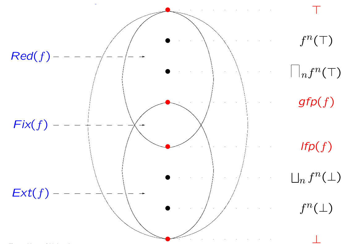
Theorem (Tarski): The set of fixpoints of a monotone function f on a complete lattice (L, \leq, \bot, \top, \sqcup, \sqcap) is a non-empty complete lattice, ordered by \leq. The least fixpoint of f is \text{lfp}(f) = \sqcap \{ x | x \geq f(x) \}, and its greatest fixpoint is \text{gfp}(f) = \sqcup \{ x | x \leq f(x) \}.
Proof: We show that a = \sqcap \{ x | f(x) \leq x \} is the least fixpoint of f. By definition, f is monotonic and a \leq x, so f(a) \leq f(x); a \in \{ x | f(x) \leq x \}, so f(a) \leq a. Then f(a) \leq \{ x | f(x) \leq x \}, so a \leq f(a). Then a = f(a), so a is a fixpoint of f. Suppose that exists another fixpoint x{}’ s.t. f(x{}’) = x{}’. Since x{}’ \in \{ x | f(x) \leq x \}, so a \leq x, then a is the least fixpoint of f. □
Equivalently, \text{lfp}(f) = \sqcap \text{Des}(f) = \sqcap \text{Fix}(f) \in \text{Fix}(f), and \text{gfp}(f) = \sqcup \text{Asc}(f) = \sqcup \text{Fix}(f) \in \text{Fix}(f).
The least fixpoint can be obtained by a transfinite iteration of f from \bot. f^{\lambda}(\bot) where \lambda is an ordinal, is defined by
f^0(\bot) = \bot f^{\lambda + 1}(\bot) = f(f^{\lambda}(\bot)) f^{\lambda} = \sqcup \{ f^\beta(\bot) | \beta \lt \lambda \}
The transfinite sequence eventually stabilizes, and its limit is \text{lfp}(f).
8.2 CPO
Definition (Chain): Let (S, \leq) be a partially ordered set. A chain C = (x_n)_{n \in \mathbb{N}} is a monotone sequence of elements of S: x_0 \leq x_1 \leq \cdots \leq x_n \leq x_{n+1} \leq \cdots.
Definition (CPO): A complete partial order is a poset (S, \leq) s.t. S has a least element \bot and every chain C has a least upper bound \sqcup C. A complete lattice is also a CPO.
Theorem (Kleene): Let (S, \leq) be a CPO. Let f: S \to S be a continuous function. Then f has a least fixpoint \text{lfp}(f) = \sqcup \{ f^i(\bot) | i \in \mathbb{N} \}.
8.3 Fixed-point Collecting Semantics
The set of reachable states can be computed as fixpoint of function next. Let F_s(S) = S_0 \cup next(S), where S_0 is the initial state. The set of reachable states is then S_r = \text{lfp}(F_s) = next^*(S_0) = \cup \{ next^*(S_0) | n \in \mathbb{N} \}.
The set of possible traces also can be computed as fixpoint. Let F_t(T) = S_0 \cup \{ t \to s{}’ | t \in T, T \text{ ends in } s, s \to s{}’ \}. The set of possible traces is T_r = \text{lfp}(F_t).
8.4 Abstraction of Fixed-points
Definition (Upper Bound Operator): An upper bound operator is a function \check{\sqcup} : L \times L \to L s.t. \forall x, y \in L, x \leq x \check{\sqcup} y and y \leq x \check{\sqcup} y.
Let (l_n)_n be a sequence of elements of L. Define the sequence (l_n^{\check{\sqcup}})_n as: l_n^{\check{\sqcup}} = \begin{cases} l_0 & \text{if } n = 0 \\ l_{n-1}^{\check{\sqcup}} \check{\sqcup} l_n & \text{if } n > 0 \end{cases}
(l_n^{\check{\sqcup}})_n is an ascending chain, and l_n^{\check{\sqcup}} \geq \{ l_0, l_1, \cdots, l_n\} for all n.
Proposition: Let F be a monotone function on a complete lattice F: L_1 \to L_1, and (\alpha, \gamma) be a Galois connection between L_1 and L_2. Then \gamma(\text{lfp}(\alpha \circ F \circ \gamma)) \geq \text{lfp}(F), i.e., \text{lfp}(\alpha \circ F \circ \gamma) \geq \alpha(\text{lfp}(F)).
8.5 Widening
Example: let int be an arbitrary fixed element of interval, then we can construct an upper bound operator:
int_1 \check{\sqcup}^{int} int_2 = \begin{cases} int_1 \sqcup int_2 & \text{if } int_1 \leq int \vee int_2 \leq int_1 \\ [-\infty, +\infty] & \text{otherwise} \end{cases}
So, [1,2] \check{\sqcup}^{[0, 2]} [2, 3] = [1, 3] (because [1,2]\leq[0,2]), and [2,3] \check{\sqcup}^{[0,2]} [1, 2] = [-\infty, +\infty] (because neither [2,3] \leq [0,2] or [1,2] \leq [0, 2]).
Definition (Widening Operator): A function \triangledown : L \times L \to L is a widening operator iff
\triangledown is an upper bound operator, i.e., \forall l_1, l_2, l_1 \leq l_1 \triangledown l_2 \wedge l2 \leq l_1 \triangledown l_2
forall ascending chains (l_n)_n the ascending chain (l_n^{\triangledown})_n eventually stablizes, where l_n^{\triangledown} = \begin{cases} l_n & \text{if } n = 0 \\ l_{n-1}^{\triangledown} \triangledown l_n & \text{otherwise} \end{cases}
Proposition: For a monotonic function f : L \to L (L is a complete lattice) and a widening operator \triangledown on L, we define the sequence (f_n^{\triangledown})_n:
f_\triangledown^n = \begin{cases} \bot & \text{if } n = 0 \\ f_{n-1}^\triangledown & \text{if } n > 0 \wedge f(f_{n-1}^\triangledown) \leq f_{n-1}^\triangledown \\ f_{n-1}^\triangledown ~ \triangledown ~ f(f_{n-1}^\triangledown) & \text{otherwise} \end{cases}
Then (f_n^{\triangledown})_n is an ascending chain and eventually stabilizes at a value f_m^{\triangledown} such that f(f_m^{\triangledown}) \leq f_m^{\triangledown}. Tarski theorem gives us f_m^\triangledown \geq \text{lfp}(f).
8.6 Narrowing
Definition (Narrowing Operator): A function \Delta : L \times L \to L is a narrowing operator iff
\Delta is a lower bound operator, i.e., \forall l_1, l_2, l_2 \leq l_1 \implies l_2 \leq l_1 \Delta l_2 \leq l_1
for all descending chains (l_n)_n (e.g., l_0 \geq l_1 \geq \cdots l_n), the descending chain x_0 = l_0, \cdots, x_{ i+1 } = x_i Δ l_{i+1} is not strictly descending.
Proposition: For a monoton function f: X \times X \to X and a narrowing operator \Delta, if x_0 \geq \text{lfp}(f) and x_0 \geq f(x_0), then the descending chain x_{i+1} = x_i \Delta f(x_i) eventually stabilizes, and its limit is greater or equal to \text{lfp}(f).
History: 2023/1 - add some left proof; 2018 - original draft