Simulating Quantum Circuits in Feynman-Style using Higher-Order Functions

In this post, we are going to build a working quantum circuit simulator (or interpreter) in Python. The simulator takes a quantum circuit program as input, and produces all possible results and their probabilities. The simulator is written in a specific style, called Feynman-style path summation, which simulates all possible worlds and calculates their contribution to the eventual result.

You do not need to understand linear algebra, Kronecker product, or matrix multiplication to understand how this quantum circuit simulator works. The only prerequisite is some Python programming and you understand the fact that functions can be used as arguments to other functions. The use of higher-order functions makes it really simple and straightforward to build a quantum circuit simulator.

from typing import Union, Callable
from dataclasses import dataclass, is_dataclass
from math import sqrt

1 Representing Quantum Circuits

The first thing is to define data structures to represent quantum circuits. Just like classical circuits, a quantum circuit consists of gates and wires connecting gates. One of the the minimal and universal set of quantum gates is the Toffoli gate plus the Hadamard gate, which are the two gates we will be implementing. With these two gates, it is possible to approximate other quantum gates with an arbitrary precision.

Exp = int | bool

The Toffoli, i.e., controlled-controlled-not (CCX) gate takes three input qubits and negates the third one if the other two controlled qubits are set. If we hardcode the first input of the CCX gate to be boolean true, then we obtain the controlled-not (CX) gate. Similarly, if we hardcode the first two inputs of CCX gate both to be boolean true, then we have the not (X) gate.

The structure of the CCX gate is simply a class with there Exps:

@dataclass
class CCX:
  x: Exp
  y: Exp
  z: Exp

The Hadamard (H) gate is something unique to quantum computing. A Hadamard gate takes a single input and creates an equal superposition of the |0⟩ and |1⟩ state. For example, if we send a classical bit through a Hadamard gate, it can be either zero or one with an equal probability. This is exactly the behavior we are going to simulate later, but now we only need to define its syntax:

@dataclass
class H:
  x: Exp

Gate = CCX | H
Circuit = list[Gate]

Let us use the Bell state🔗 as an example and see how does its circuit look like:

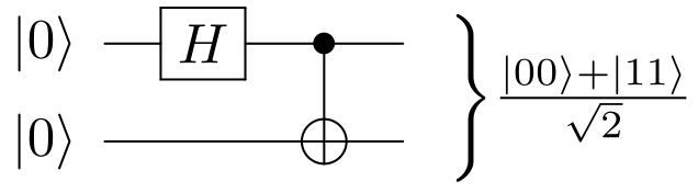
bell = [H(0), CCX(True, 0, 1)]

The circuit contains two gates, which are the H gate and CCX gate. The CCX gate has specialized its first component to boolean true, and its second and third components come from the first (0) and second (1) wire.

2 Representing Quantum States

The job of the quantum circuit simulator is to convert the input circuit to a data structure that describes the probability amplitudes of every possible resulting bit-vector state. Now, we are going to define a class that records the (classical) bit-vector bs and its probability amplitude p:

@dataclass
class State:
  p: float
  bs: tuple[bool]
  def isSet(self, x: Exp) -> bool:
    if isinstance(x, bool): return x
    return self.bs[x]

The probability amplitude is represented by a floating-point number -1.0 < p < 1.0. The bit-vector is simply a tuple of boolean values. You may see notation such as p|b_1, \dots, b_n\rangle, which is exactly what this data structure represents, where bs is a vector b_1, \dots, b_n.

There is a constraint on the probability amplitudes from the nature of quantum computation. At a certain point of simulation, there can be multiple states that are both possible. If there are n states, then the squared sum of their probability amplitudes is 1, i.e. \sum_1^{n} p_i^2 = 1.

We also define a helper function isSet that examines if an expression Exp is set in the current state. Note that since bool and int in Python are overlapped (a boolean value is also an integer value in Python), so we need to check if x is of type bool first in isSet.

Another useful helper function neg is to negate some bit given its index in the bit-vector. Since tuples are immutable in Python, we make a detour by converting to a list first and then converting back to a tuple.

def neg(bs: tuple[bool], x: int) -> tuple[bool]:
  ls = list(bs)
  ls[x] = not bs[x]
  return tuple(ls)

3 Evaluating Quantum Circuits

With the state structure defined, we can now define functions that simulate gates and circuits in quantum ways. We are going to do this step by step.

3.1 Evaluating a Single Gate

The evalGate function takes three arguments: the gate to be simulated, the current state, and a continuation. The continuation is simply a function that takes a State and returns None. In Python, we annotate its type as Callable[[State], None].

Here, we are using the power of higher-order functions: evalGate takes a function argument, representing the remaining simulation process that consumes some state.

hscale: float = 1.0 / sqrt(2.0)

def evalGate(g: Gate, s: State, k: Callable[[State], None]) -> None:
  if isinstance(g, CCX):
    if s.isSet(g.x) and s.isSet(g.y): k(State(s.p, neg(s.bs, g.z)))
    else: k(s)
  if isinstance(g, H):
    if s.isSet(g.x):
      k(State(hscale * s.p, neg(s.bs, g.x)))
      k(State(-1.0 * hscale * s.p, s.bs))
    else:
      k(State(hscale * s.p, neg(s.bs, g.x)))
      k(State(hscale * s.p, s.bs))

• If the gate is the CCX gate, we check if its first and second inputs are set (i.e. 1), since they are the control bits. If so, we invoke the continuation with a new state. This new state flips the value at the index indicated by the third input (g.z) of the CCX gate. If the first and second inputs of the CCX gate are not set, the outcome remains the same. We simply continue the evaluation by calling the continuation.

• If the gate is the Hadamard gate, we check if the only input is 1. In either case, Hadamard gate forks the simulation to two paths and we invoke the continuation twice. If b_x the input bit at index x is set, the Hadamard gate results in a superposition of \frac{1}{\sqrt{2}} s.p | b_1, \dots, !b_x, \dots, b_n\rangle and -\frac{1}{\sqrt{2}} s.p | b_1, \dots, b_x, \dots, b_n\rangle. Similarly, if b_x is not set, a superposition of \frac{1}{\sqrt{2}} s.p | b_1, \dots, !b_x, \dots, b_n\rangle and \frac{1}{\sqrt{2}} s.p | b_1, \dots, b_x, \dots, b_n\rangle is simulated. We simulate such superposition semantics by invoking the continuation twice in the program.

3.2 Evaluating Multiple Gates

Since a circuit is simply a list of gates, the evaluation of circuits is a function that structurally recurses over the list structure. The function additionally takes a state argument and a continuation function.

def evalCircuit(c: Circuit, s: State, k: Callable[[State], None]) -> None:
  if len(c) == 0: k(s)
  else: evalGate(c[0], s, lambda s: evalCircuit(c[1:], s, k))

• If the list is empty, then we apply the continuation to the current state, which means to finish the remaining computation (i.e. to summarize the result, see below).

• If the list is not empty, then we shall evaluate the first gate using evalGate under the current state, and construct a new continuation to evalGate. The content of the new continuation is to evaluate the rest of the circuit, carrying the old continuation.

3.3 Summarizing the Result

Now, you may ask what should be passed as the continuation to evalCircuit? We are going to define a “summarization” function for this purpose. The idea is to use a global mutable data structure (i.e. a mapping) to track the probability amplitudes of each final state, and this “summarization” function will properly update this data structure. In Feynman-style simulation, different simulation paths may end up with the same final state but of different probability amplitudes, and those probability amplitudes can cancel each other (remember probability amplitudes can be negative) or sum up to a larger amplitude.

summary: dict[tuple[bool], float] = {}

def summarize(s: State) -> None:
  if s.bs in summary: summary[s.bs] = summary[s.bs] + s.p
  else: summary[s.bs] = s.p

The function summarize implements what we just described. If the state has occurred in the final observation, then we sum the new probability amplitude with the accumulated one. Otherwise, we add a new observation into the mapping.

The top-level circuit evaluation is a function taking a circuit and an initial state. This function resets summary at the beginning and calls evalCircuit with function summarize as its continuation. In other words, summarize is the final halt continuation that will be invoked at the end of each path.

def runCircuit(c: Circuit, s: State) -> None:
  summary = {}
  evalCircuit(c, s, summarize)

4 Example: Bell’s State

Let us try to simulate the Bell state🔗 using the initial state |00\rangle:

runCircuit(bell, State(1.0, (False, False)))
print(summary)

The output shows two states \frac{1}{\sqrt{2}}|00\rangle and \frac{1}{\sqrt{2}}|11\rangle:

{(True, True): 0.7071067811865475, (False, False): 0.7071067811865475}

This is the expected result that the two bits are always related (identical) in the two possible outcomes.

5 Note

The continuation-based interpreter shown in this post is inspired by Choudhury et al. (2022)’s paper. They describe a Feynman-style quantum circuit interpreter using delimited continuations (shift and reset) in Racket. The interpreter is pure without using explicit mutation side effects. I also reproduced a working implementation in Scala🔗 using delimited continuations.

Aws Albarghouthi also wrote a blog post🔗 about simulating quantum circuits using linear algebra (i.e. Schrödinger-style simulation).

Bibliography

Vikraman Choudhury, Borislav Agapiev, and Amr Sabry. Scheme Pearl: Quantum Continuations. In Proc. Scheme and Functional Programming Workshop, 2022. |